20 Kolmogorov-Zurbenko filters
20.1 Background
The Kolmogorov-Zurbenko (KZ) filter is an iterative moving-average technique that separates a time series into components operating at distinct temporal scales (Zurbenko 1986; Yang and Zurbenko 2010). Its defining characteristic is simplicity: a plain moving average of window length \(m\) is applied \(k\) times in succession. This repetition transforms a box-shaped frequency response into one that closely approximates a Gaussian, attenuating high-frequency variability while preserving long-period signals with minimal distortion. The filter is written as KZ(\(m\), \(k\)), where \(m\) is the full window width in data steps (so a window of \(m = 13\) hours extends 6 hours either side of each point). The effective cut-off period (below which variation is suppressed) scales roughly as \(m\sqrt{k}\), where \(m\) is the full window width. Increasing \(k\) thus pushes the cut-off to longer periods, providing greater smoothing.
The value of the KZ filter in atmospheric and air quality science lies in the decomposition step (Rao et al. 1997; Eskridge et al. 1997). By applying the filter successively at four increasing window sizes — approximately one day, one week, one month, and one year for hourly data — and taking the differences between adjacent filtered series, the raw time series is partitioned into five additive components:
| Component | Typical period | Physical interpretation |
|---|---|---|
| Sub-day | Hours | Brief emission pulses |
| Diurnal | Diurnal cycles | Diel variation |
| Synoptic | ~1–10 days | Weather systems, regional scale episodes |
| Intermediate | Week to ~2 months | Sub-seasonal variability |
| Seasonal | Months to ~1 year | Annual cycle, photochemistry |
| Trend | Multi-year | Long-term emission changes, climate signals |
These components are mutually exclusive and sum to the original series, making the decomposition physically interpretable and suitable for downstream analysis.
The approach was first demonstrated on ambient ozone data by Rao and Zurbenko (1994) and Rao et al. (1997), who showed that synoptic-scale meteorological variability can mask long-term ozone trends unless removed. The same logic extends naturally to PM2.5, NOx, and other regulated pollutants (Wise and Comrie 2005).
By removing short-term, synoptic and seasonal variability, the KZ decomposition isolates the long-term trend component, which is often the focus of regulatory and epidemiological studies. In this respect, the filters provide a way of doing meteorological normalisation in a straightforward way, which might be useful in many settings — especially of many years of data are available. The short-term and synoptic components can be analysed separately to understand the influence of local sources and weather patterns on air quality. The intermediate component can reveal sub-seasonal phenomena such as pollution episodes or transport events.
20.2 Kolmogorov-Zurbenko Adaptive filter
The KZ Adaptive (KZA) filter extends the basic method by detecting structural breaks in the time series and shrinking the averaging window near those discontinuities (Zurbenko et al. 1996). Wherever the algorithm identifies an abrupt change — a step reduction in emissions following a policy intervention, a sensor replacement, or a sudden source change — it uses a shorter window to preserve the sharp feature rather than smearing it across a broad neighbourhood. Away from breaks the filter behaves identically to the standard KZ filter.
The degree of window shrinkage is governed by the sensitivity argument: larger values cause more aggressive adaptation. For detecting clear, sudden shifts in air quality (e.g., the introduction of a clean-air zone, COVID-19 lockdown effects, or the commissioning of an industrial scrubber) the KZA filter will generally give a cleaner result than the standard KZ filter.
20.3 Using kzFilter()
The default window sizes m = c(3, 13, 107, 721, 8761) are chosen for hourly data and correspond roughly to one day, one week, one month, and one year. The iteration count k = 5 provides a near-Gaussian frequency response at each scale. These defaults are appropriate for most ambient monitoring records and rarely need adjustment.
Different window sizes can be used for data at other time resolutions (e.g., 15-minute, daily, 1 Hz data) or to target specific temporal scales. For example, for daily data, windows of 5, 13, 41, and 365 days might be more appropriate. The key is to choose window sizes that capture the desired physical processes while ensuring sufficient data points within each window for stable averaging.
Ten years of data have been uploaded for a background (North Kensington) and roadside site (Marylebone Road) in London for 2016 to 2025, including surface meteorological data. The data can be imported as follows:
Next, we calculate the KZ components for a few pollutants at the North Kensington site. The kzFilter() function returns a data frame with the original data and new columns for each component.
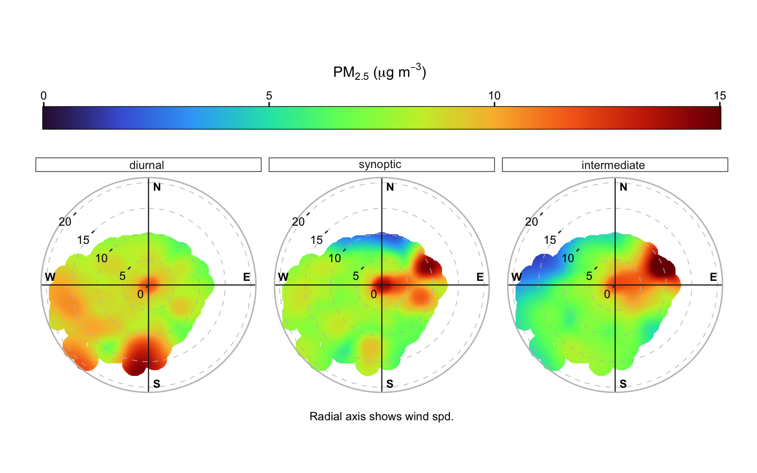
To show the different components for PM2.5, a polar plot can be produced, as shown in Figure 20.1. In this case, the diurnal, synoptic and seasonal variation are considered together. It should be noted that the trend component has been added back to show the overall variation in concentrations. The plot shows that the diurnal variation is dominated by low wind speed conditions, typical of local sources at ground level and higher wind speed features that likely reflect specific short-term source contributions. By contrast, the synoptic and intermediate variation has a much clearer easterly / north-easterly component present also at higher wind speeds, which is dominated by regional transport and the influence of pollution episodes that last a few days (synoptic) to a few weeks (intermediate).
For the synoptic / intermediate component it can be useful to plot a calendarPlot() for a particular year to highlight episodes that last days to weeks. Figure 20.2 shows the calendar plot for the synoptic + intermediate component of PM2.5 concentrations at the North Kensington site for 2020. The plot shows that the synoptic + intermediate component is dominated by a few episodes of high concentrations that last a few days and are associated with easterly / north-easterly conditions (as shown in the polar plot above). The plot also shows that there is a lot of variation in the these components, with many days having very low values, and some days having very high values. The trend component has been added back to show the overall variation in concentrations.
mutate(kz_out_pm25, episodes = synoptic + intermediate + trend) |>
  calendarPlot(
    pollutant = "episodes",
    year = 2020,
    cols = colorOpts("batlow", direction = -1),
    windflow = windflowOpts(
      colour = "white"
    )
  )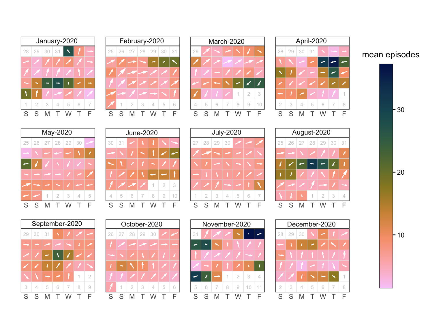
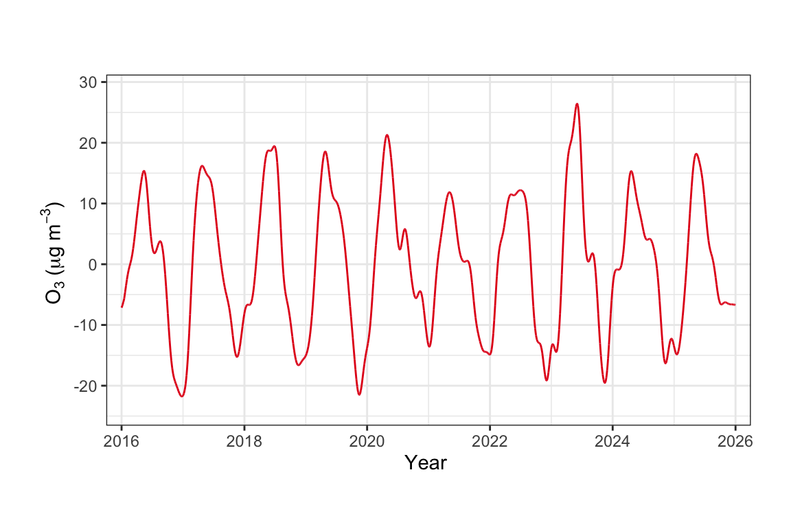
Figure 20.3 considers the seasonal component of O3 concentrations. The plot shows that the seasonal component of O3 concentrations is dominated by a strong annual cycle with high concentrations in the spring-summer and low concentrations in the winter. This is typical of O3 concentrations in urban areas, where photochemical production dominates in the summer and titration by NO dominates in the winter. Note that the seasonal component shown in Figure 20.3 is smoothly varying because the influence of shorter-term variation has been removed. It can also be useful to combine components e.g. adding the seasonal to the trend (mutate(kz_out_o3, seasonal = seasonal + trend)) to show the overall seasonal variation in concentrations on top of a long-term trend.
timePlot(
  kz_out_o3,
  pollutant = "seasonal",
  ylab = "o3 (ug/m3)",
  xlab = "Year"
)
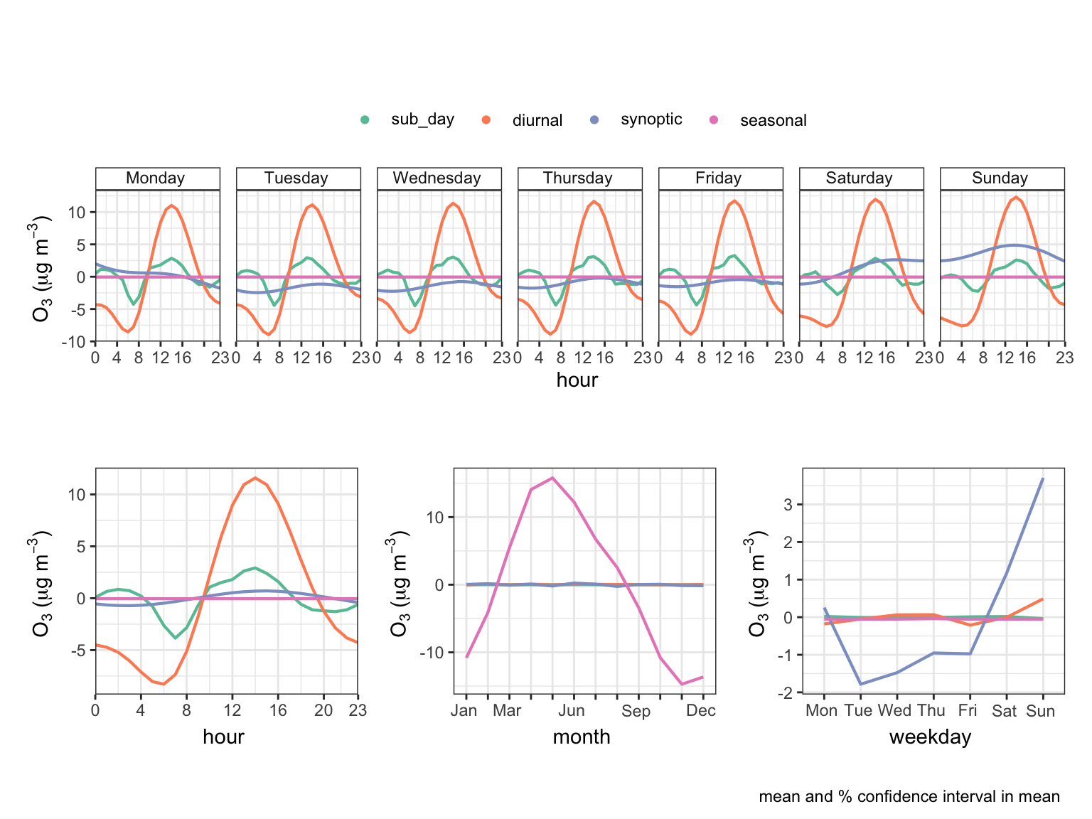
Finally, the timeVariation() function can be used to show how the different components vary by hour of the day and month of the year. Figure 20.4 shows the time variation plot for the sub-day, diurnal, synoptic and seasonal components of O3 concentrations at the North Kensington site. Figure 20.4 acts as a simple test to see which temporal variations are removed and which remain for different time scales. The sub-day component shows decrease around 7.00 to 8.00 am coinciding with the short-term morning rush hour and increased emissions of NOx that act to reduce concentrations of O3. The strong diurnal cycle with higher concentrations during the afternoon, and lower concentrations at night, shows the typical diel variation of O3 concentrations expected at an urban background site. There is no (or very little) variation in the diurnal plots for the synoptic and seasonal components because shorter-term variation has been removed.
The day of the week variation (bottom-right) shows that only synoptic component with any notable variation. In this case there are higher O3 concentrations on Saturdays and Sundays when traffic emissions of NOx are lower leading to O3 concentrations that are higher. The seasonal component shows a strong annual cycle with high concentrations in the spring-summer and low concentrations in the winter, as expected for O3 concentrations in urban areas. Similarly, there is no variation in the month of the year plot for the short-term components. These plots confirm the expected behaviour of the KZ filtering for targeted temporal scales.
timeVariation(
  kz_out_o3,
  pollutant = c("sub_day", "diurnal", "synoptic", "seasonal"),
  ci = FALSE,
  cols = "Set2",
  ylab = "o3 (ug/m3)"
)
20.4 Using kzaFilter()
kzaFilter() shares the same interface as kzFilter() with one additional argument, sensitivity, which controls how aggressively the window is reduced near structural breaks (default 1.0). It is the preferred choice when:
- A known policy change, sensor replacement, or source modification is expected to produce a step change.
- The trend component from
kzFilter()shows a suspicious sharp feature that may be an artefact of the standard window. - There is a wish to detect and locate unknown discontinuities.
The choice if kzFilter() vs kzaFilter() is often a matter of judgement and experimentation. If the KZ trend shows a sharp drop or rise, or rapid variations, that coincides with a known event, it is worth trying the KZA filter to see if it preserves that feature more cleanly. If the KZA trend is much smoother and more interpretable, it may be the better choice for subsequent analysis.
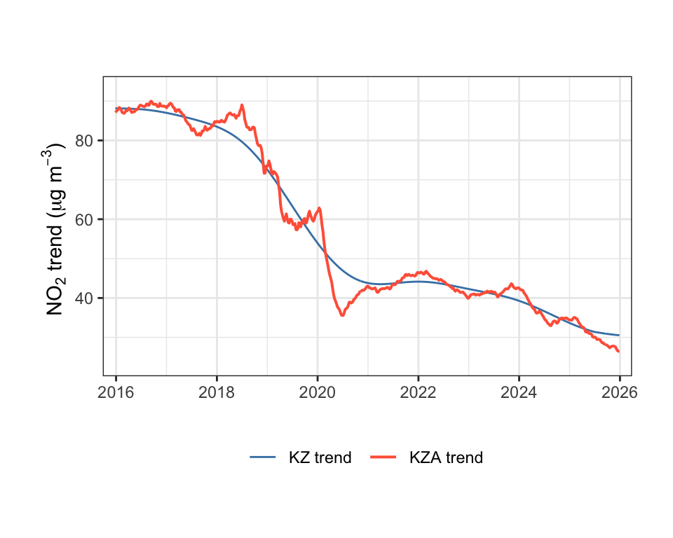
In Figure 20.5, the KZ and KZA trends for NO2 concentrations at the Marylebone Road site are compared. The KZA filter (red) preserves a sharp drop in NO2 in early 2020 that is smoothed out by the standard KZ filter (blue). This drop is related to the COVID-19 lockdown measures that were implemented in the UK in March 2020, which led to a sudden reduction in traffic emissions. The KZA filter is able to capture this abrupt change more effectively than the standard KZ filter, which smooths it out over a longer period.
trend_kz <- kzFilter(
  filter(london_aq, code == "MY1"),
  pollutant = "no2"
) |>
  rename(kz_trend = trend)

trend_kza <- kzaFilter(
  filter(london_aq, code == "MY1"),
  pollutant = "no2",
  sensitivity = 0.8
) |>
  rename(kza_trend = trend)

left_join(trend_kz, select(trend_kza, date, kza_trend), by = "date") |>
  timeAverage(avg.time = "week") |>
  timePlot(
    pollutant = c("kz_trend", "kza_trend"),
    group = TRUE,
    cols = c("steelblue", "tomato"),
    name.pol = c("KZ trend", "KZA trend"),
    ylab = "NO2 trend (ug/m3)",
    linewidth = c(0.5, 0.7)
  )
The analysis above for Covid-19 lockdown effects could arguably be better analysed by combining the seasonal and trend components using the KZ filter because the lockdown effects are not a perfect step change and and some of the effects lasted a few weeks to a few months i.e. they would be expected to also show up in the seasonal cycle. An alternative approach is shown below, but not plotted.1
Or try the
kzaFilterwithsensitivity = 0.5for more structure to capture more of the variation.↩︎