Appendix F — Openair 3.0
A major update to the openair package
Summary
Version 3 of the openair package has been released! This major update converts all plotting functions from lattice to ggplot2, among other changes. See a full list of changes here. This article describes the rationale for this change and what it means for openair users going forward.
F.1 Overview
openair 3.0 is a landmark update for the openair package, which brings a more modern plotting engine that is more flexible, customisable and extensible, and will allow openair to be developed at a greater pace and for many more years to come.
Since its inception over 10 years ago, the package has relied on lattice to produce its high quality air quality visualisations. While a very capable package, lattice is a product of its time; it is verbose, not particularly intuitive, and does not easily allow users to extend the functionality of the package. It is fair to say that it has fallen out of favour in the R community compared to ggplot2, which openair now uses.
You will still find almost all of the functions that you are used to, with some slight visual tweaks now that the new plotting engine is being used.
F.2 Benefits of ggplot2
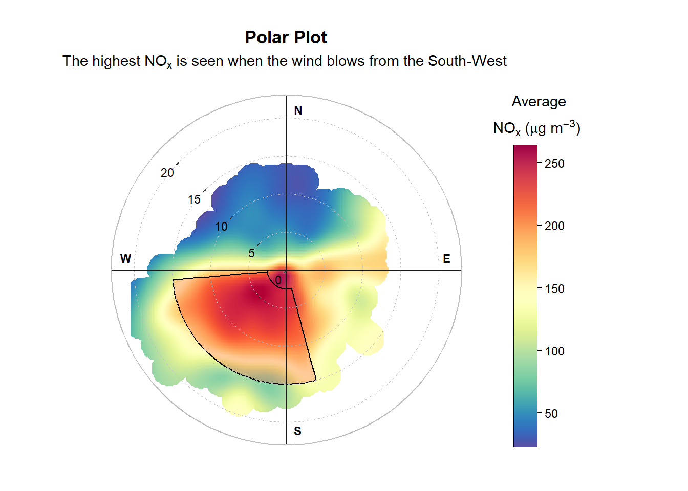
While lattice capably produced a variety of plots, once a plot was produced it was difficult to modify it after-the-fact. By comparison, ggplot2 uses a layer-based approach, meaning it is easy to layer on additional labels or annotations after a plot has been constructed.
# change some of the labels and annotate with a segment
polarplot$plot +
  ggplot2::labs(
    title = "Polar Plot",
    subtitle = quickText(
      "The highest NOx is seen when the wind blows from the South-West"
    ),
    color = quickText("Average\nNOx (ug/m3)")
  ) +
  ggplot2::annotate(
    geom = "rect",
    xmin = 165,
    xmax = 265,
    ymin = 2.5,
    ymax = 15,
    color = "black",
    fill = "red",
    alpha = 0.2
  )
Through the use of functions like ggplot2::theme(), nearly every individual visual element of a plot can be tweaked. For example, lets create a “minimalist” polarPlot() by setting a global ggplot2 theme.
# set a global ggplot2 theme
ggplot2::theme_set(ggplot2::theme_minimal())

# create a polar plot - tweaking some themes/guides afterwards
polarPlot(mydata, cols = "Blues", plot = FALSE)$plot +
  ggplot2::theme(
    panel.ontop = TRUE,
    panel.grid.minor.y = ggplot2::element_blank()
  ) +
  ggplot2::guides(
    r = ggplot2::guide_axis(angle = 0)
  )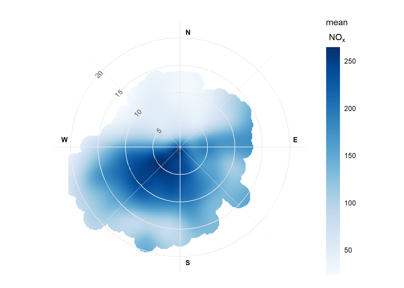
# reset theme
ggplot2::theme_set(ggplot2::theme_grey())
You can learn more about annotation in the annotation and customisation appendix.
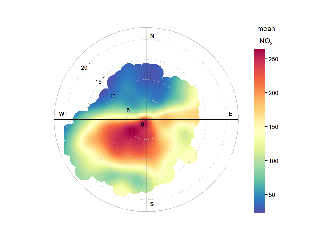
Behind-the-scenes, ggplot2 unlocks a lot of capability that was historically challenging to implement. For example, nearly all plotting functions now support two type values, meaning a 2D grid of panels can be constructed consistently across all of openair. The “polar” functions (e.g., polarPlot() and windRose()) now take advantage of native radial coordinate systems, making annotation and grid line customisation much simpler to handle without complex trigonometry. windflow has also found its way to trendLevel(), and now behaves much more consistently and flexibly across different functions. This is a taste of the many new features that will be added to the package in the coming months and years, which would have been much more difficult to implement without the switch to ggplot2.
F.3 Breaking Changes
As with any major software update, there are some ‘breaking’ changes that may affect existing code. Some of the most important are:
summaryPlot(),calcFno2()andlinearRelation()have all been removed. These functions are particularly old, behave inconsistently to the rest of the package, and haven’t been promoted in some time. It is expected that new functions will replace some of their capability in a future update. Similarly,drawOpenKey()has been removed due to no longer being necessary.Any existing lattice-based annotations may no longer work, or behave unpredictably. Any annotations are likely possible using ggplot2 functions such as
ggplot2::annotate(),ggplot2::theme()orggplot2::guides().As ggplot2 only supports a single title for its guides,
key.headerandkey.footerare deprecated in favour of a singlekey.title. If these legacy arguments are provided, they will be appended together to form the key title with a warning. This behaviour is likely to be formally removed in future.drawOpenKey()has been removed from openair due to being lattice-specific. Thekeyargument has therefore also been deprecated. To remove the legend, simply setkey.position = "none".Some arguments throughout openair have been renamed or replaced for internal consistency. For example,
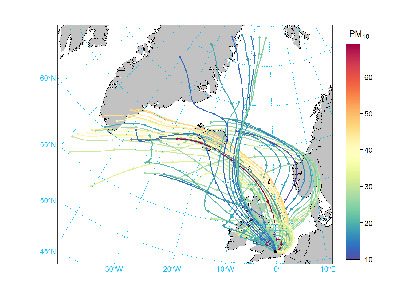
polarAnnulus()has lost thewidthargument in favour ofoffset, making it consistent withwindRose(),percentileRose()andpolarFreq().Trajectory mapping functions have been extensively rewritten, including
trajPlot(),trajLevel()andtrajCluster(). The long-term home for these functions may be in openairmaps, but for the time being they remain in openair. The previous method of map projection has been removed and replaced with an sf-powerd approach, meaning users only need to provide a “coordinate reference system” number (crs). For example, the British National Grid is ESPG:27700. As these functions no longer callscatterPlot(),scatterPlot()has lost themapargument.
While breaking changes can be frustrating, they were necessary to support the future development and maintainability of openair.
F.4 Non-Plotting Updates
While the biggest changes in openair 3.0 can be seen in the plotting functions, there are a few useful utility function updates that are important to highlight:
cutData()now possesses thedropargument, which better controls factor levels in the resulting vectors. For example, consider a dataset which only contains data for March, April, and July on whichcutData(type = "month")has been applied.drop = "empty"will return factor levels March, April and July,drop = "outside"will return March, April, May, June and July, anddrop = "none"will contain all twelve months.rollingMean()is now but one of a small family of ‘smoothing’ approaches available in openair, which now includes rolling quantiles, Gaussian smoothing, and Whittaker-Eilers smoothing. The latter is of general interest because it can be used to separate a baseline from an incremental component in a time series, which is useful for many different types of analysis e.g. better understanding local sources by considering the increment above a local background.windflowis now supported by thewindflowOpts()function, which can heavily customise the appearance of windflow arrows across all functions that support them.Many utility functions (not least
timeAverage()) are now implemented in C++, which has increased their performance massively.
F.5 Next Steps
We’d encourage you to explore what openair 3.0 has to offer.
Read the changelog to learn about all of the changes going into version 3.0.
Read the rest of the openair book; there are lots of examples of various plots in the new style.
Raise an issue if you find anything not working as it should.