Plot heat map trends

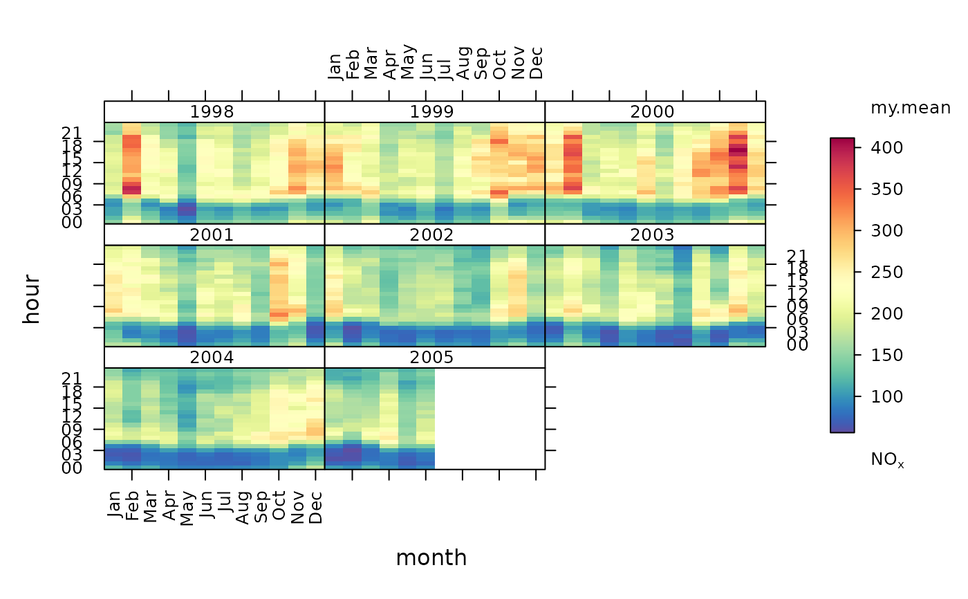
The trendLevel function provides a way of rapidly showing a large amount of data in a condensed form. In one plot, the variation in the concentration of one pollutant can to shown as a function of three other categorical properties. The default version of the plot uses y = hour of day, x = month of year and type = year to provide information on trends, seasonal effects and diurnal variations. However, x, y and type and summarising statistics can all be modified to provide a range of other similar plots.

Usage

trendLevel(
  mydata,
  pollutant = "nox",
  x = "month",
  y = "hour",
  type = "year",
  rotate.axis = c(90, 0),
  n.levels = c(10, 10, 4),
  limits = c(0, 100),
  cols = "default",
  auto.text = TRUE,
  key.header = "use.stat.name",
  key.footer = pollutant,
  key.position = "right",
  key = TRUE,
  labels = NA,
  breaks = NA,
  statistic = c("mean", "max", "min", "median", "frequency", "sum", "sd", "percentile"),
  percentile = 95,
  stat.args = NULL,
  stat.safe.mode = TRUE,
  drop.unused.types = TRUE,
  col.na = "white",
  plot = TRUE,
  ...
)

Arguments

mydata: The openair data frame to use to generate the trendLevel() plot.
pollutant: The name of the data series in mydata to sample to produce the trendLevel() plot.
x, y, type: The name of the data series to use as the trendLevel() x-axis, y-axis or conditioning variable, passed to cutData(). These are used before applying statistic. trendLevel() does not allow duplication in x, y and type options.
rotate.axis: The rotation to be applied to trendLevel x and y axes. The default, c(90, 0), rotates the x axis by 90 degrees but does not rotate the y axis. If only one value is supplied, this is applied to both axes; if more than two values are supplied, only the first two are used.
n.levels: The number of levels to split x, y and type data into if numeric. The default, c(10, 10, 4), cuts numeric x and y data into ten levels and numeric type data into four levels. This option is ignored for date conditioning and factors. If less than three values are supplied, three values are determined by recursion; if more than three values are supplied, only the first three are used.
limits: The colour scale range to use when generating the trendLevel() plot.
cols: The colour set to use to colour the trendLevel() surface. cols is passed to openColours() for evaluation.
auto.text: Automatic routine text formatting. auto.text = TRUE passes common lattice labelling terms (e.g. xlab for the x-axis, ylab for the y-axis and main for the title) to the plot via quickText() to provide common text formatting. The alternative auto.text = FALSE turns this option off and passes any supplied labels to the plot without modification.
key.header, key.footer: Adds additional text labels above and/or below the scale key, respectively. For example, passing the options key.header = "", key.footer = c("mean","nox") adds the addition text as a scale footer. If enabled (auto.text = TRUE), these arguments are passed to the scale key (drawOpenKey()) via quickText() to handle formatting. The term "get.stat.name", used as the default key.header setting, is reserved and automatically adds statistic function names or defaults to "level" when unnamed functions are requested via statistic.
key.position: Location where the scale key should be plotted. Allowed arguments currently include "top", "right", "bottom", and "left".
key: Fine control of the scale key via drawOpenKey().
breaks, labels: If a categorical colour scale is required then breaks should be specified. These should be provided as a numeric vector, e.g., breaks = c(0, 50, 100, 1000). Users should set the maximum value of breaks to exceed the maximum data value to ensure it is within the maximum final range, e.g., 100–1000 in this case. Labels will automatically be generated, but can be customised by passing a character vector to labels, e.g., labels = c("good", "bad", "very bad"). In this example, 0 - 50 will be "good" and so on. Note there is one less label than break.
statistic: The statistic to apply when aggregating the data; default is the mean. Can be one of "mean", "max", "min", "median", "frequency", "sum", "sd", "percentile". Note that "sd" is the standard deviation, "frequency" is the number (frequency) of valid records in the period and "data.cap" is the percentage data capture. "percentile" is the percentile level (%) between 0-100, which can be set using the "percentile" option. Functions can also be sent directly via statistic; see 'Details' for more information.
percentile: The percentile level used when statistic = "percentile". The default is 95%.
stat.args: Additional options to be used with statistic if this is a function. The extra options should be supplied as a list of named parameters; see 'Details' for more information.
stat.safe.mode: An addition protection applied when using functions directly with statistic that most users can ignore. This option returns NA instead of running statistic on binned sub samples that are empty. Many common functions terminate with an error message when applied to an empty dataset. So, this option provides a mechanism to work with such functions. For a very few cases, e.g., for a function that counted missing entries, it might need to be set to FALSE; see 'Details' for more information.
drop.unused.types: Hide unused/empty type conditioning cases. Some conditioning options may generate empty cases for some data sets, e.g. a hour of the day when no measurements were taken. Empty x and y cases generate 'holes' in individual plots. However, empty type cases would produce blank panels if plotted. Therefore, the default, TRUE, excludes these empty panels from the plot. The alternative FALSE plots all type panels.
col.na: Colour to be used to show missing data.
plot: Should a plot be produced? FALSE can be useful when analysing data to extract plot components and plotting them in other ways.
...: Addition options are passed on to cutData() for type handling and lattice::levelplot() for finer control of the plot itself.

Value

an openair object.

Details

trendLevel() allows the use of third party summarising functions via the statistic option. Any additional function arguments not included within a function called using statistic should be supplied as a list of named parameters and sent using stat.args. For example, the encoded option statistic = "mean" is equivalent to statistic = mean, stat.args = list(na.rm = TRUE) or the R command mean(x, na.rm = TRUE). Many R functions and user's own code could be applied in a similar fashion, subject to the following restrictions: the first argument sent to the function must be the data series to be analysed; the name 'x' cannot be used for any of the extra options supplied in stat.args; and the function should return the required answer as a numeric or NA. Note: If the supplied function returns more than one answer, currently only the first of these is retained and used by trendLevel(). All other returned information will be ignored without warning. If the function terminates with an error when it is sent an empty data series, the option stat.safe.mode should not be set to FALSE or trendLevel() may fail. Note: The stat.safe.mode = TRUE option returns an NA without warning for empty data series.

Author

Karl Ropkins

David Carslaw

Jack Davison

Examples

# basic use
# default statistic = "mean"
trendLevel(mydata, pollutant = "nox")


# applying same as 'own' statistic
my.mean <- function(x) mean(x, na.rm = TRUE)
trendLevel(mydata, pollutant = "nox", statistic = my.mean)


# alternative for 'third party' statistic
# trendLevel(mydata, pollutant = "nox", statistic = mean,
#           stat.args = list(na.rm = TRUE))

if (FALSE) { # \dontrun{
# example with categorical scale
trendLevel(mydata,
  pollutant = "no2",
  border = "white", statistic = "max",
  breaks = c(0, 50, 100, 500),
  labels = c("low", "medium", "high"),
  cols = c("forestgreen", "yellow", "red")
)
} # }